Linear Regression Using MLIB
This article was published as a part of the Data Science Blogathon.
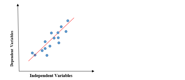
Introduction to Linear Regression
In this article we will be learning about the Linear Regression using MLIB and everything will be hands-on i.e. we will be building an end to end Linear regression model which will predict the customer’s yearly spend on the company’s product if we talk about the dataset so it is completely a dummy dataset which is generated in purpose to understand the concepts of model building for continuous data using “MLIB”.
Mandatory Steps for Linear Regression using MLIB
Before getting into the machine learning process and following the steps to predict the customer’s yearly spending we must need to initialize the Spark Session and read our dummy dataset of e-commerce websites that have all the relevant features.
- Initializing the Spark Session
- Reading the dataset
Setting up the spark session
In this particular section, we will setup up the Spark object so that we will be able to create an environment to perform the operations which are supported and managed by it.
from pyspark.sql import SparkSession
spark = SparkSession.builder.appName('E-commerce').getOrCreate()
Inference: So from the above two code lines we have successfully imported the SparkSession object from PySpark’s SQL package and then we have created the environment using the getOrCreate() function one thing to note is that before creating it we have built it using the builder function and given it the name as “E-commerce”
Reading the dataset
In this section, we will be reading the dummy dataset which I’ve created to perform the ML operations along with Data Preprocessing using PySpark.
data = spark.read.csv("Ecommerce_Customers.csv",inferSchema=True,header=True)
Inference: So in the above line of code we have read the Ecommerce data and kept the inferSchema parameter as True so that it will return the real data type that which dataset possesses and the header as True so that the first tuple of record will be stated as header.
Showing the Schema of our dataset
Here the Schema of the dataset will be shown so that one could get the inference of what kind of data each column holds and then the analysis could be done with more precision.
data.printSchema()
Output:
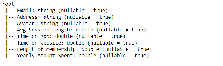
Inference: So we have used the printSchema() function to show the information about each column that our dataset holds and while looking at the output one can see what kind of data type is there.
Now we will go through the dataset using three different ways so that one could also know all the methods to investigate it.
- show() function
- head() function
- Iterating through each item
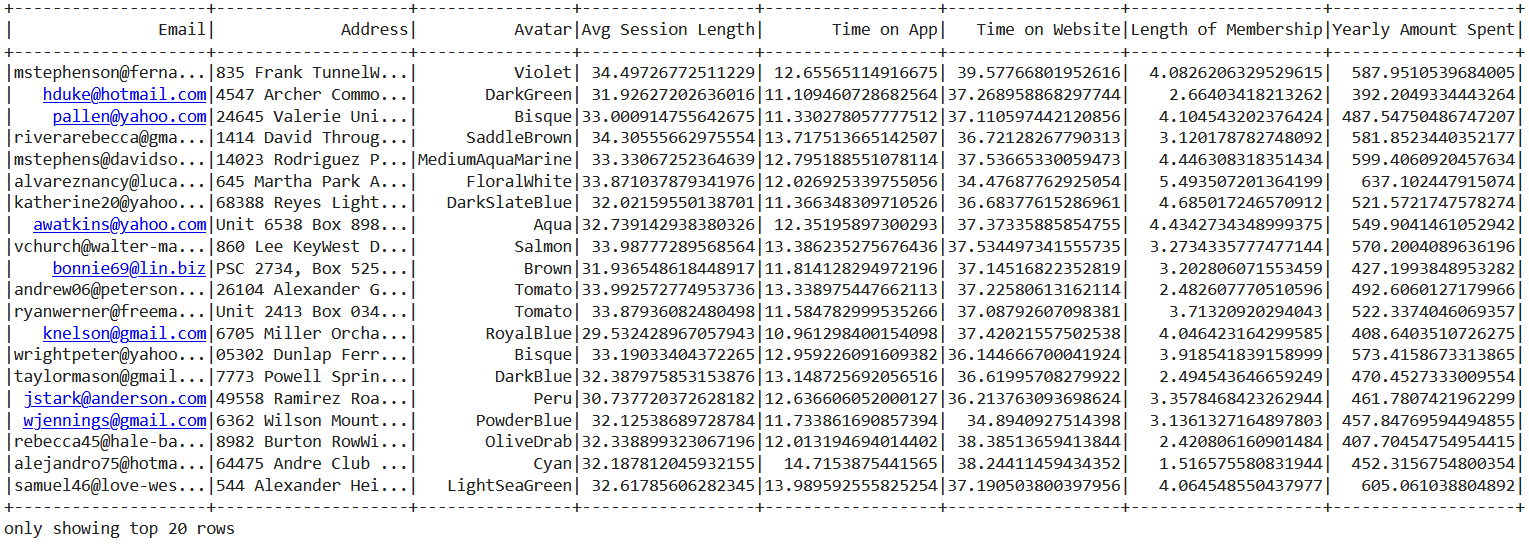
Looking at the data using the show() function where it will return the top 20 rows from the complete data.
Now the head function needs to be introduced which is quite similar to the head function used in pandas in the below code’s output we can see that the head function returned the Row object which holds one complete record/tuple.
data.head()
Output:
Row(Email='[email protected]', Address='835 Frank TunnelWrightmouth, MI 82180-9605', Avatar='Violet', Avg Session Length=34.49726772511229, Time on App=12.65565114916675, Time on Website=39.57766801952616, Length of Membership=4.0826206329529615, Yearly Amount Spent=587.9510539684005)
Now let’s see the more clear version of getting into the data where each item will be iterable through the combination of for loop and head function and the output shown is the more clear version of the Row object output.
for item in data.head():
    print(item)
Output:
[email protected]
835 Frank TunnelWrightmouth, MI 82180-9605
Violet
34.49726772511229
12.65565114916675
39.57766801952616
4.0826206329529615
587.9510539684005
Importing Linear Regression Library
As mentioned earlier that we will gonna predict the customer’s yearly expenditure on products so based on what we already know, we have to deal with continuous data and when we are working with such type of data we have to use the linear regression model.
For that reason, we will be importing the Linear Regression package from the ML library of PySpark.
from pyspark.ml.regression import LinearRegression
Data Preprocessing for Machine Learning
In this section, all the data preprocessing techniques will be performed which are required to make the dataset ready to be sent across the ML pipeline where the model could easily adapt and build an efficient model.
Importing Vector and VectorAssembler libraries so that we could easily separate the features columns and the Label column i.e. all the dependent columns will be stacked together as the feature column and the independent column will be as a label column.
from pyspark.ml.linalg import Vectors
from pyspark.ml.feature import VectorAssembler
Let’s have a look at which columns are present in our dataset.
data.columns
Output:
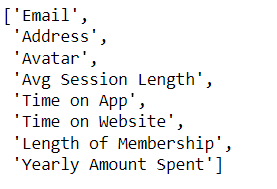
Inference: So from the above output all the columns are listed down in the form of list type only but this will not give us enough information about which column to select hence for that reason we will use the describe method.
data.describe()
Output:
DataFrame[summary: string, Email: string, Address: string, Avatar: string, Avg Session Length: string, Time on App: string, Time on Website: string, Length of Membership: string, Yearly Amount Spent: string]
Inference: If you will go through the output closely you will find that columns that have a string as the data type will have no role in the model development phase as machine learning is the involvement of mathematical calculation where only number game is allowed hence integer and double data type columns accepted.
Based on the above discussion the columns which are selected to be part of the machine learning pipeline are as follows:
- Average Session Length
- Time on App
- Time on Website
- Length of Membership
assembler = VectorAssembler(
    inputCols=["Avg Session Length", "Time on App",
               "Time on Website",'Length of Membership'],
    outputCol="features")
Output:
Inference: In the above code we chose the VectorAssembler method to stack all our features columns together and return them as the “features” columns by the output column parameter.
output = assembler.transform(data)
Here, the Transform function is used to fit the real data with the changes that we have done in the assembler variable using the VectorAssembler function so that the changes should reflect in the real dataset.
output.select("features").show()
Output:
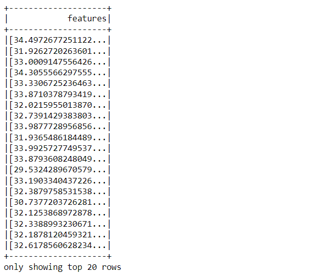
Now with the select function, we have selected only the features column from the dataset and showed it in the form of DataFrame using the show() function.
final_data = output.select("features",'Yearly Amount Spent')
From the above code, we are concatenating the stack of dependent features (named as features) and independent features together and naming it final_data and this frame will be analyzed further in the process.
Train Test Split
In this step of the model building, we will be dividing our data into a training set and the testing set, where training data will be the one on top of which our model will be built and on the other hand testing data is the one on which we will test our model that how well it performed.
In MLIB, for dividing the data into testing and training sets we have to use a random split() function which takes an input in the form of the list type.
train_data,test_data = final_data.randomSplit([0.7,0.3])
Inference: With the help of the tuple unpacking concept we have stored the training set (70%) into train_data and similarly 30% of the dataset into test_data. Note that in the random split() method the list is passed.
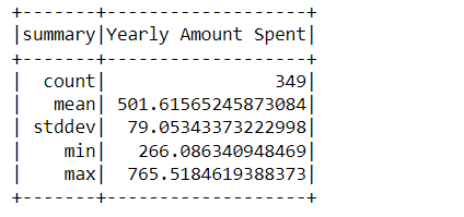
train_data.describe().show()
Output:
test_data.describe().show()
Output:
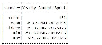
Inference: Describe method seems to be an accurate way to analyze and draw the difference between training and testing data where we can see that in the training set there are 349 records while 151 are on the other hand.
Model Development
Finally, we have come across the step where we will be building our Linear Regression Model and for that LinearRegression object is used which if you remember we have imported in the starting and then passed the “Yearly Amount Spent” column in the label Column parameter which is our independent column.
lr = LinearRegression(labelCol='Yearly Amount Spent')
Now, as we have created our Linear Regression object so now we can easily fit our data i.e. we can do the model training by passing the training data in the fit method.
lrModel = lr.fit(train_data,)
Now, let’s print the Coefficients of each feature and intercepts of the model which is being trained on the training dataset this is also one of the pieces of information which will let you know how well your model is involving each independent variable separately.
print("Coefficients: {} Intercept: {}".format(lrModel.coefficients,lrModel.intercept))
Output:
Coefficients: [25.324513354618116,38.880247333555445,0.20347373150823037,61.82593066961652] Intercept: -1031.8607952442187
Model Evaluation
So in this step, we will be evaluating our model i.e. We will analyze how well our model performed, and in this stage of the model building, we decide whether to go with the existing one or not in the model deployment stage.
So for evaluation, we have come across the “evaluate” function and stored it in the test_results variable as we will use it for further analysis.
test_results = lrModel.evaluate(test_data)
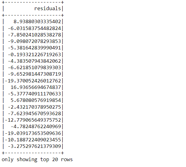
The one who knows the mathematical intuition behind Linear Regression must be aware of the fact that residual = Original result – Predicted result i.e. the difference between the predicted result by the model and the original result of the label column.
test_results.residuals.show()
Output:
Now it’s time to make predictions from our model for that we will first store the unlabelled data i.e the feature data and transform it too so that changes will take place.
unlabeled_data = test_data.select('features')

predictions = lrModel.transform(unlabeled_data)
predictions.show()
Output:
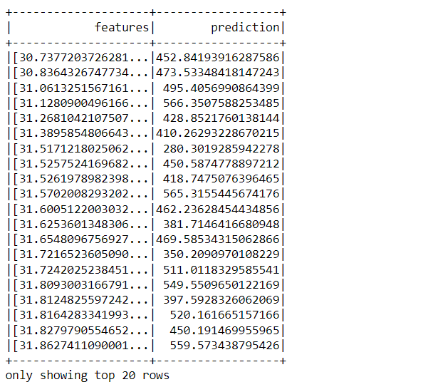
Inference: So from the above output we can see that it returned a DataFrame that practically has two columns one is the complete stack of features column and the other one is the prediction column.
Conclusion
So, in this section we will see by far what we have learned in this article if I have to mention it in the nutshell then we have gone through a complete machine learning pipeline for the linear regression algorithm.
- We started the spark session and read the dataset on top of which everything was performed.
- Then we performed each data preprocessing step which was required to make the data ready for an ML algorithm to accept.
- After Data cleaning we moved towards dividing the data and later towards the model building where we built a Linear regression model.
- In the end, we evaluated the model using relevant functions and predicted the results.
Here’s the repo link to this article. I hope you liked my article on Introduction to Linear Regression using MLIB. If you have any opinions or questions, then comment below.
Connect with me on LinkedIn for further discussion.
The media shown in this article is not owned by Analytics Vidhya and is used at the Author’s discretion.


