µTransfer: A technique for hyperparameter tuning of enormous neural networks

Great scientific achievements cannot be made by trial and error alone. Every launch in the space program is underpinned by centuries of fundamental research in aerodynamics, propulsion, and celestial bodies. In the same way, when it comes to building large-scale AI systems, fundamental research forms the theoretical insights that drastically reduce the amount of trial and error necessary and can prove very cost-effective. 

In this post, we relay how our fundamental research enabled us, for the first time, to tune enormous neural networks that are too expensive to train more than once. We achieved this by showing that a particular parameterization preserves optimal hyperparameters across different model sizes. This is the µ-Parametrization (or µP, pronounced “myu-P”) that we introduced in a previous paper, where we showed that it uniquely enables maximal feature learning in the infinite-width limit. In collaboration with researchers at OpenAI, we verified its practical advantage on a range of realistic scenarios, which we describe in our new paper, “Tensor Programs V: Tuning Large Neural Networks via Zero-Shot Hyperparameter Transfer.”

By greatly reducing the need to guess which training hyperparameters to use, this technique can accelerate research on enormous neural networks, such as GPT-3 (opens in new tab) and potentially larger successors in the future. We also released a PyTorch package that facilitates the integration of our technique in existing models, available on the project GitHub page (opens in new tab) or by simply running \(\texttt{pip install mup}\).

“µP provides an impressive step toward removing some of the black magic from scaling up neural networks. It also provides a theoretically backed explanation of some tricks used by past work, like the T5 model (opens in new tab). I believe both practitioners and researchers alike will find this work valuable.”

— Colin Raffel, Assistant Professor of Computer Science, University of North Carolina at Chapel Hill and co-creator of T5

Scaling the initialization is easy, but scaling training is hard

Large neural networks are hard to train partly because we don’t understand how their behavior changes as their size increases. Early work on deep learning, such as by Glorot & Bengio and He et al., generated useful heuristics that deep learning practitioners widely use today. In general, these heuristics try to keep the activation scales consistent at initialization. However, as training starts, this consistency breaks at different model widths, as illustrated on the left in Figure 1.

Unlike at random initialization, behavior during training is much harder to mathematically analyze. Our goal is to obtain a similar consistency so that as model width increases, the change in activation scales during training stay consistent and similar to initialization to avoid numerical overflow and underflow. Our solution, µP, achieves this goal, as seen on the right in Figure 1, which shows the stability of network activation scales for the first few steps of training across increasing model width. 

Our parameterization, which maintains this consistency during training, follows two pieces of crucial insight. First, gradient updates behave differently from random weights when the width is large. This is because gradient updates are derived from data and contain correlations, whereas random initializations do not. Therefore, they need to be scaled differently. Second, parameters of different shapes also behave differently when the width is large. While we typically divide parameters into weights and biases, with the former being matrices and the latter vectors, some weights behave like vectors in the large-width setting. For example, the embedding matrix in a language model is of size vocabsize x width. While the width tends to infinity, vocabsize stays constant and finite. During matrix multiplication, the difference in behavior between summing along a finite dimension and an infinite one cannot be more different.

These insights, which we discuss in detail in a previous blog post, motivated us to develop µP. In fact, beyond just keeping the activation scale consistent throughout training, µP ensures that neural networks of different and sufficiently large widths behave similarly during training such that they converge to a desirable limit, which we call the feature learning limit. 

A theory-guided approach to scaling width

Our theory of scaling enables a procedure to transfer training hyperparameters across model sizes. If, as discussed above, µP networks of different widths share similar training dynamics, they likely also share similar optimal hyperparameters. Consequently, we can simply apply the optimal hyperparameters of a small model directly onto a scaled-up version. We call this practical procedure µTransfer. If our hypothesis is correct, the training loss-hyperparameter curves for µP models of different widths would share a similar minimum.

Conversely, our reasoning suggests that no scaling rule of initialization and learning rate other than µP can achieve the same result. This is supported by the animation below. Here, we vary the parameterization by interpolating the initialization scaling and the learning rate scaling between PyTorch default and µP. As shown, µP is the only parameterization that preserves the optimal learning rate across width, achieves the best performance for the model with width 213 = 8192, and where wider models always do better for a given learning rate—that is, graphically, the curves don’t intersect. 

Building on the theoretical foundation of Tensor Programs, µTransfer works automatically for advanced architectures, such as Transformer and ResNet. It can also simultaneously transfer a wide range of hyperparameters. Using Transformer as an example, we demonstrate in Figure 3 how the optima of key hyperparameters are stable across widths. 

(opens in new tab)

“I am excited about µP advancing our understanding of large models. µP’s principled way of parameterizing the model and selecting the learning rate make it easier for anybody to scale the training of deep neural networks. Such an elegant combination of beautiful theory and practical impact.”

— Johannes Gehrke, Technical Fellow, Lab Director of Research at Redmond, and CTO and Head of Machine Learning for the Intelligent Communications and Conversations Cloud (IC3)

Beyond width: Empirical scaling of model depth and more

Modern neural network scaling involves many more dimensions than just width. In our work, we also explore how µP can be applied to realistic training scenarios by combining it with simple heuristics for nonwidth dimensions. In Figure 4, we use the same transformer setup to show how the optimal learning rate remains stable within reasonable ranges of nonwidth dimensions. For hyperparameters other than learning rate, see Figure 19 in our paper. 

(opens in new tab)

Testing µTransfer

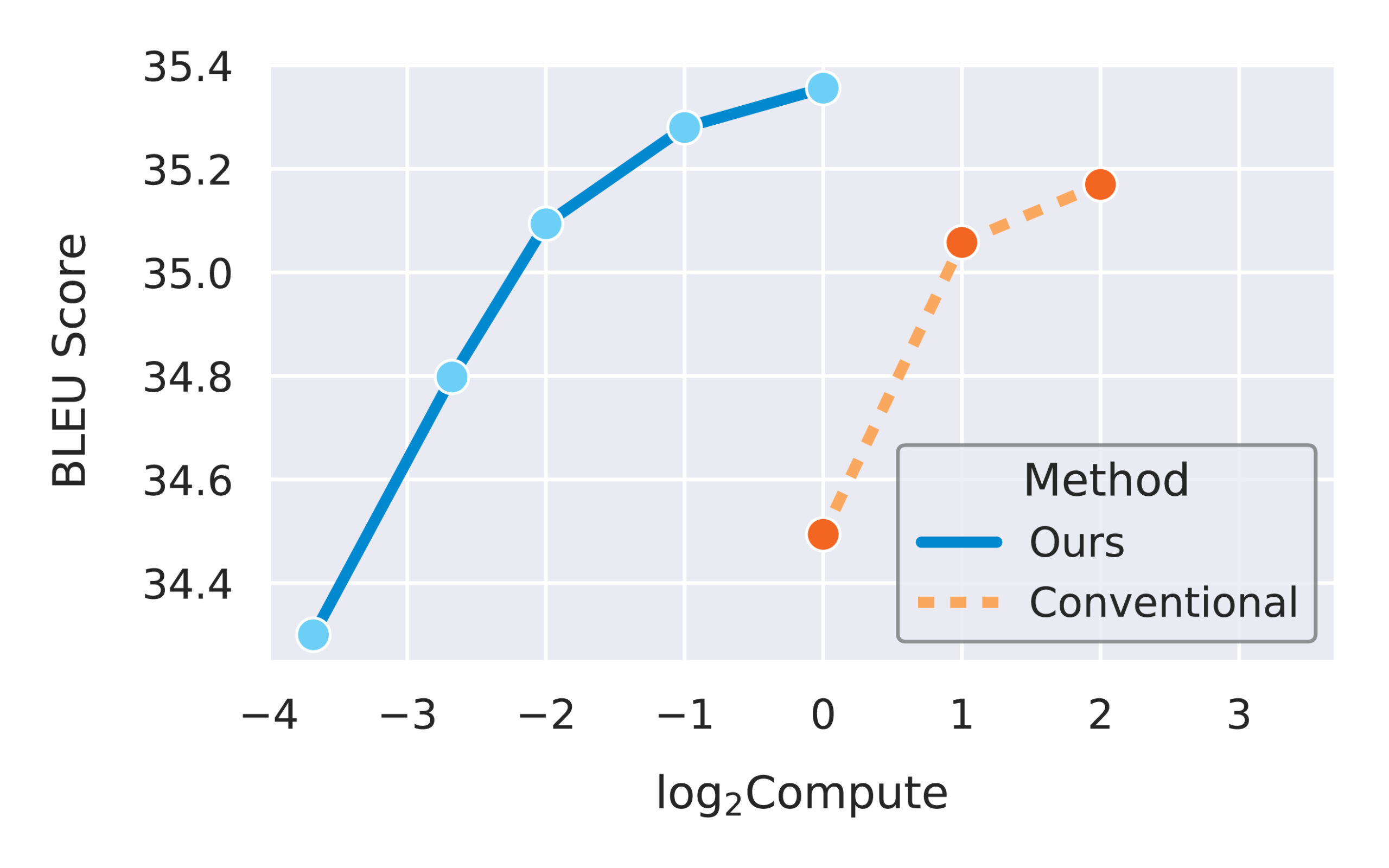
Now that we have verified the transfer of individual hyperparameters, it is time to combine them in a more realistic scenario. In Figure 5, we compare µTransfer, which transfers tuned hyperparameters from a small proxy model, with directly tuning the large target model. In both cases, the tuning is done via random search. Figure 5 illustrates a Pareto frontier (opens in new tab) of the relative tuning compute budget compared with the tuned model quality (BLEU score) on IWSLT14 De-En (opens in new tab), a machine translation dataset. Across all compute budget levels, µTransfer is about an order of magnitude (in base 10) more compute-efficient for tuning. We expect this efficiency gap to dramatically grow as we move to larger target model sizes. 

A glimpse of the future: µP + GPT-3

Before this work, the larger a model was, the less well-tuned we expected it to be due to the high cost of tuning. Therefore, we expected that the largest models could benefit the most from µTransfer, which is why we partnered with OpenAI to evaluate it on GPT-3. 

After parameterizing a version of GPT-3 with relative attention in µP, we tuned a small proxy model with 40 million parameters before copying the best hyperparameter combination to the 6.7-billion parameter variant of GPT-3, as prescribed by µTransfer. The total compute used during this tuning stage was only 7 percent of the compute used in the pretraining of the final 6.7-billion model. This µTransferred model outperformed the model of the same size (with absolute attention) in the original GPT-3 paper (opens in new tab). In fact, it performs similarly to the model (with absolute attention) with double the parameter count from the same paper, as shown in Figure 6. 

(opens in new tab)

Implications for deep learning theory

As shown previously, µP gives a scaling rule which uniquely preserves the optimal hyperparameter combination across models of different widths in terms of training loss. Conversely, other scaling rules, like the default in PyTorch or the NTK parameterization (opens in new tab) studied in the theoretical literature, are looking at regions in the hyperparameter space farther and farther from the optimum as the network gets wider. In that regard, we believe that the feature learning limit of µP, rather than the NTK limit (opens in new tab), is the most natural limit to study if our goal is to derive insights that are applicable to feature learning neural networks used in practice. As a result, more advanced theories on overparameterized neural networks should reproduce the feature learning limit of µP in the large width setting. 

Theory of Tensor Programs

The advances described above are made possible by the theory of Tensor Programs (TPs) developed over the last several years. Just as autograd helps practitioners compute the gradient of any general computation graph, TP theory enables researchers to compute the limit of any general computation graph when its matrix dimensions become large. Applied to the underlying graphs for neural network initialization, training, and inference, the TP technique yields fundamental theoretical results, such as the architectural universality of the Neural Network-Gaussian Process correspondence and the Dynamical Dichotomy theorem, in addition to deriving µP and the feature learning limit that led to µTransfer. Looking ahead, we believe extensions of TP theory to depth, batch size, and other scale dimensions hold the key to the reliable scaling of large models beyond width. 

Applying µTransfer to your own models

Even though the math can be intuitive, we found that implementing µP (which enables µTransfer) from scratch can be error prone. This is similar to how autograd is tricky to implement from scratch even though the chain rule for taking derivatives is very straightforward. For this reason, we created the mup package (opens in new tab) to enable practitioners to easily implement µP in their own PyTorch models, just as how frameworks like PyTorch, TensorFlow, and JAX have enabled us to take autograd for granted. Please note that µTransfer works for models of any size, not just those with billions of parameters. 

The journey has just begun

While our theory explains why models of different widths behave differently, more investigation is needed to build a theoretical understanding of the scaling of network depth and other scale dimensions. Many works have addressed the latter, such as the research on batch size by Shallue et al. (opens in new tab), Smith et al. (opens in new tab), and McCandlish et al. (opens in new tab), as well as research on neural language models in general by Rosenfield et al. (opens in new tab) and Kaplan et al. (opens in new tab) We believe µP can remove a confounding variable for such investigations.  Furthermore, recent large-scale architectures often involve scale dimensions beyond those we have talked about in our work, such as the number of experts in a mixture-of-experts system. Another high-impact domain to which µP and µTransfer have not been applied is fine tuning a pretrained model. While feature learning is crucial in that domain, the need for regularization and the finite-width effect prove to be interesting challenges. 

We firmly believe in fundamental research as a cost-effective complement to trial and error and plan to continue our work to derive more principled approaches to large-scale machine learning. To learn about our other deep learning projects or opportunities to work with us and even help us expand µP, please go to our Deep Learning Group page.

Opens in a new tab