Implementing Audio Classification Project Using Deep Learning

This article was published as a part of the Data Science Blogathon.

Hello all, welcome to a wonderful article where we will be exploring learnings for audio and sound classification using Machine learning and deep learning. It is amazing and interesting to know – how machines are capable of understanding human language, and responding in the same way. NLP(Natural Language Processing) is one of the most researched and studied topics of today’s generation, it helps to make machines capable of handling human language in the form of speech as well as text.

Table of Contents

1. Introduction to Audio Classification
2. Project Overview
3. Dataset Overview
4. Hands-on Implementing Audio Classification project
   • EDA On Audio Data
   • Data Preprocessing
   • Building ANN for Audio Classification
   • Testing some unknown Audio
5. End Notes

Introduction to Audio Classification

Audio Classification means categorizing certain sounds in some categories, like environmental sound classification and speech recognition. The task we perform same as in Image classification of cat and dog, Text classification of spam and ham. It is the same applied in audio classification. The only difference is the type of data where we have images, text, and now we have a certain type of audio file of a certain length.

Why Audio Classification is termed as difficult than other types of classification?

There are many techniques to classify images as we have different in-built neural networks under CNN, especially to deal with images. And it is easy to extract features from images because images already come in the form of numbers, as the formation of an image is a collection of pixels, and pixels are in the form of numbers. When we have data as text, we use the sequential encoder and decoder-based techniques to find features. But when the buzzing is about recognizing speech, it becomes difficult to compare it to text because it is based on frequency and time. So you need to extract proper pitch and frequency.

Audio classification employs in industries across different domains like voice lock features, music genre identification, Natural Language classification, Environment sound classification, and to capture and identify different types of sound. It is used in chatbots to provide chatbots with the next level of power.

Project Overview

Sound classification is a growing area of research that everyone is trying to learn and implement on some kinds of projects. The project we will build in this article is simply such that a beginner can easily follow – where the problem statement to apply the deep learning techniques to classify environmental sounds, specifically focusing on identifying the urban sounds.

Given an audio sample of some category with a certain duration in .wav extension and determine whether it contains target urban sounds. It lies under the supervised machine learning category, so we have a dataset as well as a target category.

Dataset Overview

The dataset we will use is called as Urban Sound 8k dataset. The dataset contains 8732 sound files of 10 different classes and is listed below. Our task is to extract different features from these files and classify the corresponding audio files into respective categories. You can download the dataset from the official website from here, and it is also available on Kaggle. The size of the dataset is a little bit large, so if it’s not possible to download, then you can create Kaggle Notebook and can practice it on Kaggle itself.

• Air Conditioner
• Car Horn
• Children Playing
• Dog Bark
• Drilling Machine
• Engine Idling
• Gun Shot
• Jackhammer
• Siren
• Street Music

Hands-On Practice of Audio Classification Project

Libraries Installation

The very important and great library that supports audio and music analysis is Librosa. Simply use the Pip command to install the library. It provides building blocks that are required to construct an information retrieval model from music. Another great library we will use is for deep learning modeling purposes is TensorFlow, and I hope everyone has already installed TensorFlow.

pip install librosa
pip install tensorflow

Exploratory Data Analysis of Audio data

We have 10 different folders under the urban dataset folder. Before applying any preprocessing, we will try to understand how to load audio files and how to visualize them in form of the waveform. If you want to load the audio file and listen to it, then you can use the IPython library and directly give it an audio file path. We have taken the first audio file in the fold 1 folder that belongs to the dog bark category.

import IPython.display as ipd
filepath = "../input/urbansound8k/fold1/101415-3-0-2.wav"
ipd.Audio(filepath)

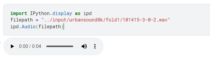
Image Source – screenshot by Author

Now we will use Librosa to load audio data. So when we load any audio file with Librosa, it gives us 2 things. One is sample rate, and the other is a two-dimensional array. Let us load the above audio file with Librosa and plot the waveform using Librosa.

• Sample rate – It represents how many samples are recorded per second. The default sampling rate with which librosa reads the file is 22050. The sample rate differs by the library you choose.
• 2-D Array – The first axis represents recorded samples of amplitude. And the second axis represents the number of channels. There are different types of channels – Monophonic(audio that has one channel) and stereo(audio that has two channels).

import librosa
import librosa.display
data, sample_rate = librosa.load(filepath)
plt.figure(figsize=(12, 5))
librosa.display.waveshow(data, sr=sample_rate)

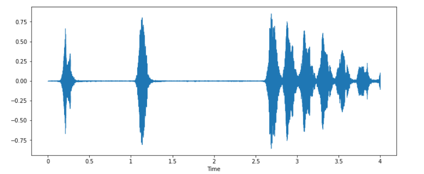
As we read, if you try to print the sample rate, then it’s output will be 22050 because when we load the data with librosa, then it normalizes the entire data and tries to give it in a single sample rate. The same we can achieve using scipy python library also. It will also give us two pieces of information – one is sample rate, and the other is data.

When you print the sample rate using scipy-it is different than librosa. Now let us visualize the wave audio data. One important thing to understand between both is- when we print the data retrieved from librosa, it can be normalized, but when we try to read an audio file using scipy, it can’t be normalized. Librosa is now getting popular for audio signal processing because of the following three reasons.

1. It tries to converge the signal into mono(one channel).
2. It can represent the audio signal between -1 to +1(in normalized form), so a regular pattern is observed.
3. It is also able to see the sample rate, and by default, it converts it to 22 kHz, while in the case of other libraries, we see it according to a different value.

Imbalance Dataset check

Now we know about the audio files and how to visualize them in audio format. Moving format to data exploration we will load the CSV data file provided for each audio file and check how many records we have for each class.

import pandas as pd
metadata = pd.read_csv('/urbansound8k/UrbanSound8K.csv')
metadata.head(10)

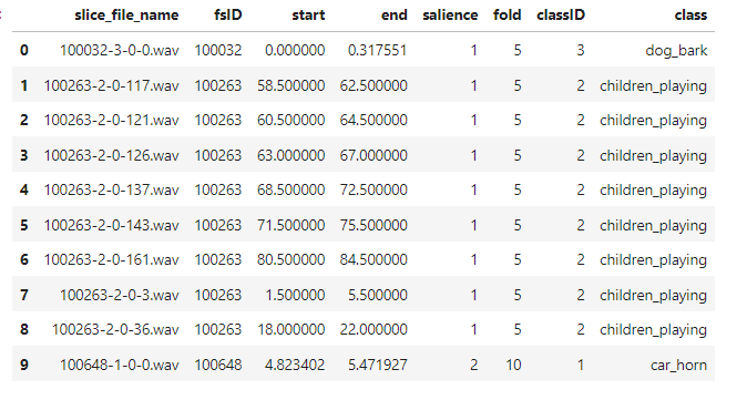
The data we have is a filename and where it is present so let us explore 1st file, so it is present in fold 5 with category as a dog bark. Now use the value counts function to check records of each class.

metadata['class'].value_counts()

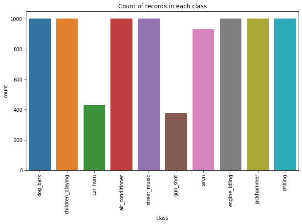
When you see the output so data is not imbalanced, and most of the classes have an approximately equal number of records. We can also visualize the count of records in each category using a bar plot or count plot.

import seaborn as sns
plt.figure(figsize=(10, 6))
sns.countplot(metadata['class'])
plt.title("Count of records in each class")
plt.xticks(rotation="vertical")
plt.show()

Data Preprocessing

Some audios are getting recorded at a different rate-like 44KHz or 22KHz. Using librosa, it will be at 22KHz, and then, we can see the data in a normalized pattern. Now, our task is to extract some important information, and keep our data in the form of independent(Extracted features from the audio signal) and dependent features(class labels). We will use Mel Frequency Cepstral coefficients to extract independent features from audio signals.

MFCCs – The MFCC summarizes the frequency distribution across the window size. So, it is possible to analyze both the frequency and time characteristics of the sound. This audio representation will allow us to identify features for classification. So, it will try to convert audio into some kind of features based on time and frequency characteristics that will help us to do classification. To know and read more about MFCC, you can watch this video and can also read this research paper by springer.

To demonstrate how we apply MFCC in practice, first, we will apply it on a single audio file that we are already using.

mfccs = librosa.feature.mfcc(y=data, sr=sample_rate, n_mfcc=40)
print(mfccs.shape)
print(mfccs)

👉Now, we have to extract features from all the audio files and prepare the dataframe. So, we will create a function that takes the filename(file path where it is present). It loads the file using librosa, where we get 2 information. First, we’ll find MFCC for the audio data, And to find out scaled features, we’ll find the mean of the transpose of an array.

def features_extractor(file):
    #load the file (audio)
    audio, sample_rate = librosa.load(file_name, res_type='kaiser_fast') 
    #we extract mfcc
    mfccs_features = librosa.feature.mfcc(y=audio, sr=sample_rate, n_mfcc=40)
    #in order to find out scaled feature we do mean of transpose of value
    mfccs_scaled_features = np.mean(mfccs_features.T,axis=0)
    return mfccs_scaled_features

👉 Now, to extract all the features for each audio file, we have to use a loop over each row in the dataframe. We also use the TQDM python library to track the progress. Inside the loop, we’ll prepare a customized file path for each file and call the function to extract MFCC features and append features and corresponding labels in a newly formed dataframe.

#Now we ned to extract the featured from all the audio files so we use tqdm
import numpy as np
from tqdm import tqdm
### Now we iterate through every audio file and extract features 
### using Mel-Frequency Cepstral Coefficients
extracted_features=[]
for index_num,row in tqdm(metadata.iterrows()):
    file_name = os.path.join(os.path.abspath(audio_dataset_path),'fold'+str(row["fold"])+'/',str(row["slice_file_name"]))
    final_class_labels=row["class"]
    data=features_extractor(file_name)
    extracted_features.append([data,final_class_labels])

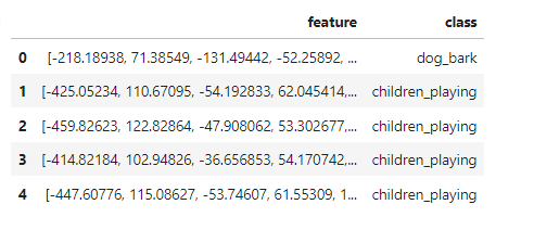
The loop will take a little bit of time to run because it will iterate over 8000 rows, and after that, you can observe the dataframe of extracted features as shown below.

### converting extracted_features to Pandas dataframe
extracted_features_df=pd.DataFrame(extracted_features,columns=['feature','class'])
extracted_features_df.head()

 

Train Test split

First, we split the dependent and independent features. After that, we have 10 classes, so we use label encoding(Integer label encoding) from number 1 to 10 and convert it into categories. After that, we split the data into train and test sets in an 80-20 ratio.

### Split the dataset into independent and dependent dataset
X=np.array(extracted_features_df['feature'].tolist())
y=np.array(extracted_features_df['class'].tolist())
### Label Encoding -> Label Encoder
from tensorflow.keras.utils import to_categorical
from sklearn.preprocessing import LabelEncoder
labelencoder=LabelEncoder()
y=to_categorical(labelencoder.fit_transform(y))
### Train Test Split
from sklearn.model_selection import train_test_split
X_train,X_test,y_train,y_test=train_test_split(X,y,test_size=0.2,random_state=0)

Totally, we have 6985 records in the train set and 1747 samples in the test set. Let’s head over to Model creation.

Audio Classification Model Creation

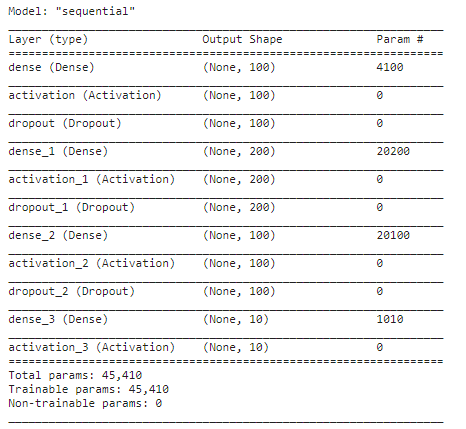
We have extracted features from the audio sample and splitter in the train and test set. Now we will implement an ANN model using Keras sequential API. The number of classes is 10, which is our output shape(number of classes), and we will create ANN with 3 dense layers and architecture is explained below.

1. The first layer has 100 neurons. Input shape is 40 according to the number of features with activation function as Relu, and to avoid any overfitting, we’ll use the Dropout layer at a rate of 0.5.
2. The second layer has 200 neurons with activation function as Relu and the drop out at a rate of 0.5.
3. The third layer again has 100 neurons with activation as Relu and the drop out at a rate of 0.5.

from tensorflow.keras.models import Sequential
from tensorflow.keras.layers import Dense,Dropout,Activation,Flatten
from tensorflow.keras.optimizers import Adam
from sklearn import metrics
### No of classes
num_labels=y.shape[1]

model=Sequential()
###first layer
model.add(Dense(100,input_shape=(40,)))
model.add(Activation('relu'))
model.add(Dropout(0.5))
###second layer
model.add(Dense(200))
model.add(Activation('relu'))
model.add(Dropout(0.5))
###third layer
model.add(Dense(100))
model.add(Activation('relu'))
model.add(Dropout(0.5))
###final layer
model.add(Dense(num_labels))
model.add(Activation('softmax'))

👉 You can observe the model summary using the summary function.

Compile the Model

To compile the model we need to define loss function which is categorical cross-entropy, accuracy metrics which is accuracy score, and an optimizer which is Adam.

model.compile(loss='categorical_crossentropy',metrics=['accuracy'],optimizer='adam')

Train the Model

We will train the model and save the model in HDF5 format. We will train a model for 100 epochs and batch size as 32. We’ll use callback, which is a checkpoint to know how much time it took to train over data.

## Trianing my model
from tensorflow.keras.callbacks import ModelCheckpoint
from datetime import datetime 
num_epochs = 100
num_batch_size = 32
checkpointer = ModelCheckpoint(filepath='./audio_classification.hdf5', 
                               verbose=1, save_best_only=True)
start = datetime.now()
model.fit(X_train, y_train, batch_size=num_batch_size, epochs=num_epochs, validation_data=(X_test, y_test), callbacks=[checkpointer], verbose=1)
duration = datetime.now() - start
print("Training completed in time: ", duration)

Check the Test Accuracy

Now we will evaluate the model on test data. we got near about 77 percent accuracy on the training dataset and 76 percent on test data.

test_accuracy=model.evaluate(X_test,y_test,verbose=0)
print(test_accuracy[1])

If you are using the TensorFlow version below 2.6, then you can use predict classes function to predict the corresponding class for each audio file. But, if you are using 2.6 and above, then you can use predict and argument maximum function.

#model.predict_classes(X_test)
predict_x=model.predict(X_test) 
classes_x=np.argmax(predict_x,axis=1)
print(classes_x)

Testing Some Test Audio Sample

Now it is time to test some random audio samples. Whenever we’ll get new audio, we have to perform three steps again to get the predicted label and class.

1. First, preprocess the audio file (load it using Librosa and extract MFCC features)
2. Predict the label to which audio belongs.
3. An inverse transforms the predicted label to get the respective class name to which it belongs.

filename="../input/urbansound8k/fold7/101848-9-0-0.wav"
#preprocess the audio file
audio, sample_rate = librosa.load(filename, res_type='kaiser_fast') 
mfccs_features = librosa.feature.mfcc(y=audio, sr=sample_rate, n_mfcc=40)
mfccs_scaled_features = np.mean(mfccs_features.T,axis=0)
#Reshape MFCC feature to 2-D array
mfccs_scaled_features=mfccs_scaled_features.reshape(1,-1)
#predicted_label=model.predict_classes(mfccs_scaled_features)
x_predict=model.predict(mfccs_scaled_features) 
predicted_label=np.argmax(x_predict,axis=1)
print(predicted_label)
prediction_class = labelencoder.inverse_transform(predicted_label) 
print(prediction_class)

Conclusion

Congratulations! 👏 If you have followed the article till here and have tried to implement it along with the reading. Then, you have learned how to deal with the audio data and use MFCC to extract important features from audio samples and build a simple ANN model on top of it to classify the audio in a different class. To practice this project, I am providing you with the environmental sound classification dataset present over Kaggle and trying to implement this project for practice purposes. The learning of this article can be concluded in some bullet points as discussed below.

• Audio classification is a technique to classify sounds into different categories.
• We can visualize any audio in the form of a waveform.
• MFCC method is used to extract important features from audio files.
• Scaling the audio samples to a common scale is important before feeding data to the model to understand it better.
• You can build a CNN model to classify audios. And as well as try to build a much deeper ANN than we have built.

👉 The complete Notebook implementation is available here.

👉 I hope that each step was easy to catch and follow. If you have any queries on the audio classification project, then feel free to post them in the comment section below. And you can also connect with me.

👉 Connect with me on Linkedin.

👉 Check out my other articles on Analytics Vidhya and crazy-techie

Thanks for giving your time!

The media shown in this article is not owned by Analytics Vidhya and are used at the Author’s discretion. 

Raghav Agrawal 07 Apr 2022

I am a final year undergraduate who loves to learn and write about technology. I am a passionate learner, and a data science enthusiast. I am learning and working in data science field from past 2 years, and aspire to grow as Big data architect.